
InfluxDB is an open-source database optimized for time-series data. Its core design goal is to efficiently store and query timestamped metric data (such as monitoring data, sensor readings, application performance metrics, etc.).
In the field of web crawlers, it is mainly used for real-time monitoring of crawler running status, helping developers dynamically track crawling efficiency, exceptions, and resource consumption.
- Server monitoring:
CPU usage,memory occupancy,network traffic - IoT sensors:
temperature,humidity,device status - Application performance:
API response time,error rate,request volume
Stock data is naturally time-series data, with data in different cycles such as milliseconds, minutes, hours, and days. It is also very suitable for storage using InfluxDB.
InfluxDB Comparison with Traditional Solutions (e.g., MySQL)
| Requirement | InfluxDB | MySQL |
|---|---|---|
| Write 100,000 market quotes per second | ✅ Native support for high-concurrency writes | ❌ Requires database and table partitioning + queue buffering |
| Calculate the 5-day moving average of 500 stocks | ✅ Millisecond-level response (optimized by time window functions) | ❌ Complex SQL + indexing, with second-level latency |
| Store 10 years of historical data | ✅ Automatic compression and downsampling (saves 90% of space) | ❌ Raw data expands, and query speed slows down |
| Real-time monitoring of price fluctuations | ✅ Stream processing + instant alerts (integrated with Kapacitor) | ❌ Depends on an external computing framework |
Now, let’s start a hands-on, zero-based tutorial on InfluxDB to get you up and running with InfluxDB in the shortest possible time. We’ll crawl stock data, store it in InfluxDB, and then query the data.
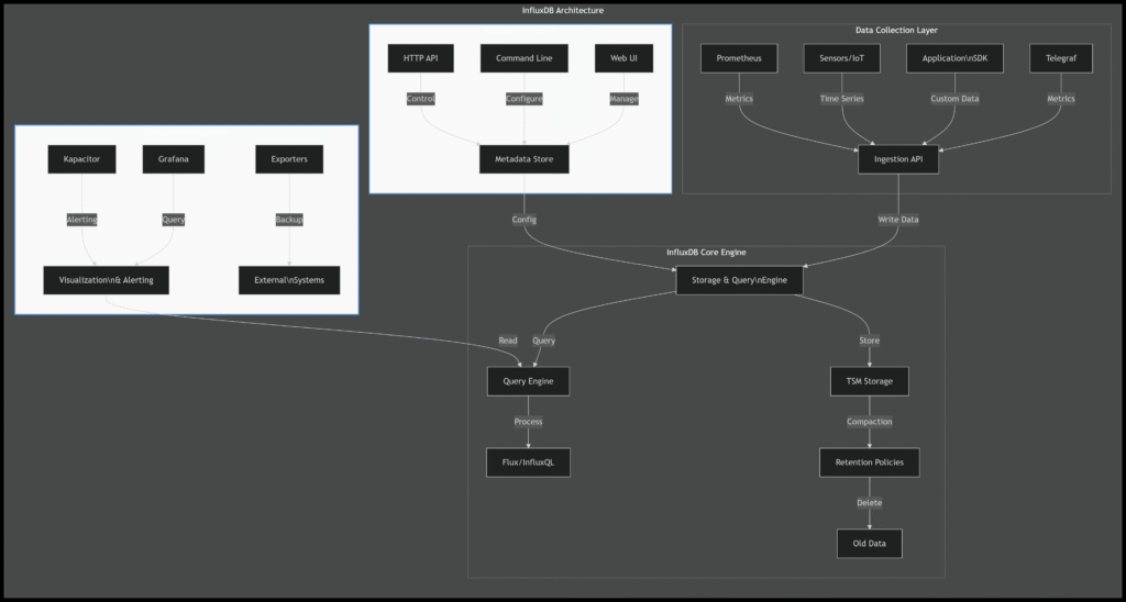
InfluxDB Architecture Diagram
Installation
InfluxDB supports Windows, Linux, and macOS operating systems.
This article uses Ubuntu as an example to introduce its installation and usage tutorials.
$ wget https://dl.influxdata.com/influxdb/releases/influxdb_1.8.10_amd64.debWait a moment to get the downloaded installation package.
sudo dpkg -i influxdb_1.8.10_amd64.debThe output result is as follows:
Selecting previously unselected package influxdb.
(Reading database ... 33306 files and directories currently installed.)
Preparing to unpack influxdb_1.8.10_amd64.deb ...
Unpacking influxdb (1.8.10-1) ...
Setting up influxdb (1.8.10-1) ...
Created symlink /etc/systemd/system/influxd.service → /lib/systemd/system/influxdb.service.
Created symlink /etc/systemd/system/multi-user.target.wants/influxdb.service → /lib/systemd/system/influxdb.service.
Start InfluxDB.
sudo systemctl start influxdbTest if the installation was successful.
influx -versionOutput:
InfluxDB shell version: 1.8.10You can enter the database by typing influx.
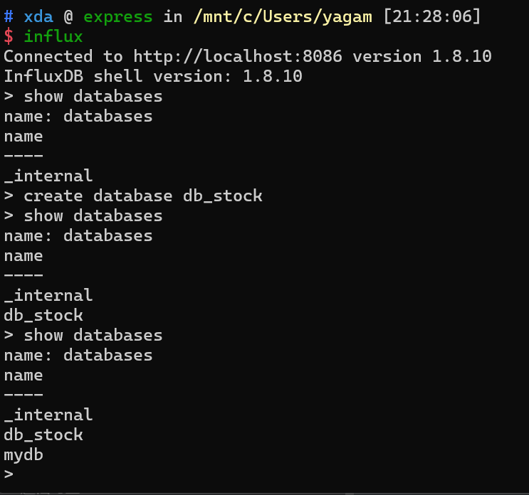
Create a database:
CREATE DATABASE db_stockDisplay all databases.
SHOW DATABASES;Notice that its syntax is very similar to that of MySQL.
It also provides a RESTFUL API for access.
For example, the above method of creating a database can be achieved through the API.
curl -X POST "http://localhost:8086/query" --data-urlencode "q=CREATE DATABASE db_stock"InfluxDB opens port 8086 by default for HTTP access.
InfluxDB does not require pre-creating Measurements: When writing data for the first time, InfluxDB will automatically create the corresponding Measurement.
And dynamically add Tags and Fields: New Tags or Fields can be dynamically added each time data is written without prior definition.
Now that our InfluxDB is ready, let’s retrieve stock data from the internet.
Python Web Crawler to Retrieve US Stock Data
We are now going to retrieve minute-by-minute data for US stocks.
We’ll use Sina’s data source:
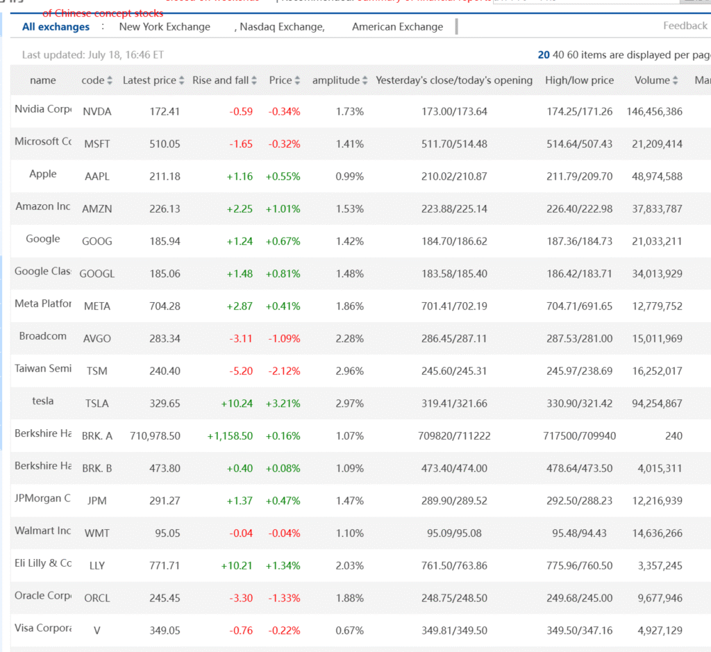
crawler source as below:
import pandas as pd
import requests

proxy_host = {'http':'https://api.2808proxy.com/proxy'} # use proxy if web block ip

def stock_us_daily(symbol: str = "FB", adjust: str = "") -> pd.DataFrame:
    """
    Sina Finance - U.S. Stocks
    https://finance.sina.com.cn/stock/usstock/sector.shtml
    Remark:
    1. CIEN Sina's ex-rights and ex-dividends factor is incorrect.
    2. AI The Sina reweighting factor is incorrect. This stock has just been listed and no reweighting has occurred, yet a reweighting factor is returned.
    :param symbol: stock symbol
    :type symbol: str
    :param adjust: "": Returns unadjusted data; qfq: Returns data after forward adjustment; qfq-factor: Returns forward adjustment factors and adjustments;
    :type adjust: str
    :return:  adjusted data
    :rtype: pandas.DataFrame
    """
    url = f"https://finance.sina.com.cn/staticdata/us/{symbol}"
    res = requests.get(url,proxx=proxy_host)
    js_code = py_mini_racer.MiniRacer()
    js_code.eval(zh_js_decode)
    dict_list = js_code.call("d", res.text.split("=")[1].split(";")[0].replace('"', ""))
    data_df = pd.DataFrame(dict_list)
    data_df["date"] = pd.to_datetime(data_df["date"]).dt.date
    data_df.index = pd.to_datetime(data_df["date"])
    del data_df["amount"]
    del data_df["date"]
    data_df = data_df.astype("float")
    url = us_sina_stock_hist_qfq_url.format(symbol)
    res = requests.get(url)
    qfq_factor_df = pd.DataFrame(eval(res.text.split("=")[1].split("\n")[0])["data"])
    qfq_factor_df.rename(
        columns={
            "c": "adjust",
            "d": "date",
            "f": "qfq_factor",
        },
        inplace=True,
    )
    qfq_factor_df.index = pd.to_datetime(qfq_factor_df["date"])
    del qfq_factor_df["date"]

    # process reweighting factor
    temp_date_range = pd.date_range("1900-01-01", qfq_factor_df.index[0].isoformat())
    temp_df = pd.DataFrame(range(len(temp_date_range)), temp_date_range)
    new_range = pd.merge(
        temp_df, qfq_factor_df, left_index=True, right_index=True, how="left"
    )
    new_range = new_range.ffill()
    new_range = new_range.iloc[:, [1, 2]]

    if adjust == "qfq":
        if len(new_range) == 1:
            new_range.index.values[0] = pd.to_datetime(str(data_df.index.date[0]))
        temp_df = pd.merge(
            data_df, new_range, left_index=True, right_index=True, how="left"
        )
        try:
            # try for pandas >= 2.1.0
            temp_df.ffill(inplace=True)
        except Exception:
            try:
                # try for pandas < 2.1.0
                temp_df.fillna(method="ffill", inplace=True)
            except Exception as e:
                print("Error:", e)
        try:
            # try for pandas >= 2.1.0
            temp_df.bfill(inplace=True)
        except Exception:
            try:
                # try for pandas < 2.1.0
                temp_df.fillna(method="bfill", inplace=True)
            except Exception as e:
                print("Error:", e)

        temp_df = temp_df.astype(float)
        temp_df["open"] = temp_df["open"] * temp_df["qfq_factor"] + temp_df["adjust"]
        temp_df["high"] = temp_df["high"] * temp_df["qfq_factor"] + temp_df["adjust"]
        temp_df["close"] = temp_df["close"] * temp_df["qfq_factor"] + temp_df["adjust"]
        temp_df["low"] = temp_df["low"] * temp_df["qfq_factor"] + temp_df["adjust"]
        temp_df = temp_df.apply(lambda x: round(x, 4))
        temp_df = temp_df.astype("float")
        # process reweighting factor error - start
        check_df = temp_df[["open", "high", "low", "close"]].copy()
        check_df.dropna(inplace=True)
        if check_df.empty:
            data_df.reset_index(inplace=True)
            return data_df
        # process reweighting factor error - finish
        result_data = temp_df.iloc[:, :-2]
        result_data.reset_index(inplace=True)
        return result_data

    if adjust == "qfq-factor":
        qfq_factor_df.reset_index(inplace=True)
        return qfq_factor_df

    if adjust == "":
        data_df.reset_index(inplace=True)
        return data_df
This time, we’ll retrieve data for NVIDIA stocks.
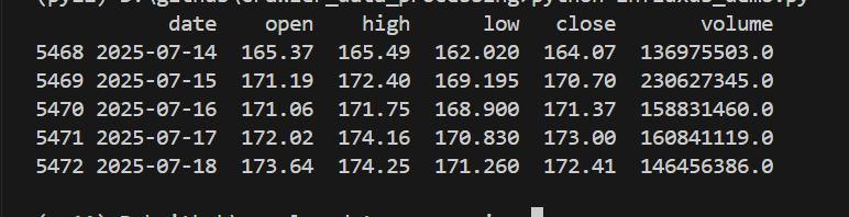
def fetch_stock_data(ticker):

    df = stock_us_daily(symbol=ticker)  # NVIDIA stock history data
    print(df.tail())


if __name__== '__main__':
    fetch_stock_data("NVDA")
The output is as follows:
Next, we’ll write the data to InfluxDB.
The input parameter is a DataFrame, which will be converted to a list.
# connect to InfluxDB
client = InfluxDBClient(host='localhost', port=8086)
client.switch_database('db_stock')


def write_data_to_influx_db(df):

    date_column = 'date'
    # make sure date column is datetime type
    if not pd.api.types.is_datetime64_any_dtype(df[date_column]):
        df[date_column] = pd.to_datetime(df[date_column])
    df['symbol'] = 'NVDA'
    # set date column as index
    points = []
    for _, row in df.iterrows():
        point = {
            "measurement": "stock_data",  # measurement is like a table in SQL
            "time": row["date"],
            "tags": {
                "ticker": row["symbol"]  # ticker is like a column in SQL
            },
            "fields": {
                "open": row["open"],
                "close": row["close"],
                "high": row["high"],
                "low": row["low"],
                "volume": row["volume"]

            }
        }
        points.append(point)

    try:
        client.write_points(
            points=points,
            time_precision='s'
        )
    except Exception as e:
        print(f"Error writing data: {e}")
    finally:
        client.close()
Note the distinction between tags and fields here.
In InfluxDB, a tag is metadata used for indexing and classifying data. It is one of the core components of the time-series data model and is mainly used to improve query efficiency and data filtering capabilities.
Core Features of Tags
- String Type
Tag values can only be strings and do not support other types such as numerical or boolean values. For example,symbol="AAPL"(stock code) andexchange="NASDAQ"(stock exchange) are typical tags. - Indexed
InfluxDB automatically creates an index for tags. Therefore, queries based on tags (such as filtering and grouping) are extremely fast, making them suitable for high-frequency screening scenarios. - Used for Classification and Dimension Division Tags are usually used to represent the “dimensions” or “attributes” of data and are used to distinguish data from different sources, types, or categories. For example:
- In stock data,
symbol(stock code) andmarket(market) can be used as tags to distinguish different stocks. - In sensor data,
device_id(device ID) andlocation(location) can be used as tags to distinguish different devices.
The difference between tags and fields: In InfluxDB, data consists of a measurement (similar to a table name), tags, fields, and a timestamp. The differences between tags and fields are as follows:
| Feature | Tag | Field |
|---|---|---|
| Data Type | Only strings | Supports numerical values, strings, booleans, etc. |
| Indexed | Yes (fast query speed) | No (slower query speed) |
| Purpose | Used for filtering, grouping, and classifying data | Used to store actual measurement values (such as stock prices and trading volumes) |
| Storage Occupancy | Indexing increases storage overhead | No indexing, more efficient storage |
After running the Python program, let’s enter InfluxDB to check the data.
select * from stock_dataThe query statement is exactly the same as that in MySQL. The measurement defined above is used as the table name. So, those familiar with MySQL can master the CRUD operations in InfluxDB without any barriers.
The result is as follows:
Connected to http://localhost:8086 version 1.8.10
InfluxDB shell version: 1.8.10
> use db_stock
Using database db_stock
> select * from stock_data
name: stock_data
name: stock_data
time                close   high     low      open    ticker volume
----                -----   ----     ---      ----    ------ ------
1727654400000000000 121.44  121.5    118.15   118.31  NVDA   227053651
1727740800000000000 117     122.4351 115.79   121.765 NVDA   302094485
1727827200000000000 118.85  119.38   115.14   116.44  NVDA   221845872
1727913600000000000 122.85  124.36   120.3401 120.92  NVDA   277117973
1728000000000000000 124.92  125.04   121.83   124.94  NVDA   244465552
1728259200000000000 127.72  130.64   124.95   124.99  NVDA   346250233
1728345600000000000 132.89  133.48   129.42   130.26  NVDA   285722485
1728432000000000000 132.65  134.52   131.38   134.11  NVDA   246191561
1728518400000000000 134.81  135      131      131.91  NVDA   242311332
....... ignore multiple lines
Of course, it’s more common to use the API to retrieve data.
def query_data_from_influx_db():
    query = 'SELECT * FROM stock_data WHERE ticker = \'NVDA\' ORDER BY time DESC'
    result = client.query(query)
    df = pd.DataFrame(list(result.get_points()))
    print(df.head())

if __name__ == '__main__':
    # df = fetch_stock_data("NVDA")
    # write_data_to_influx_db(df)
    query_data_from_influx_db()
Then we can retrieve the daily data to calculate the MA moving average.
df = pd.DataFrame(list(result.get_points()))
df['time'] = pd.to_datetime(df['time'])
df.set_index('time', inplace=True)

# 2. calculate  avg 5day's price
df['ma5'] = df['close'].rolling(window=5).mean()
print(df[['close', 'ma5']].tail(10))- The core usage methods of stock data after being stored in InfluxDB include:
- Basic Queries: Use InfluxQL to extract raw data such as K-line and trading volume.
- Analysis and Calculation: Combine with Python to calculate technical indicators (such as moving averages and MACD).
- Visualization: Display trend charts through Grafana.
- Real-time Monitoring: Write programs to implement price alerts and anomaly detection.
- Performance Optimization: Use continuous queries to pre-calculate high-frequency indicators.